Table of Contents
- 1. Structure of Scheduling Algorithms
- 2. List of Algorithms
- 3. Algorithm for Problem 1|rj|Cmax
- 4. Bratley’s Algorithm
- 5. Hodgson's Algorithm
- 6. Algorithm for Problem P||Cmax
- 7. McNaughton's Algorithm
- 8. Algorithm for Problem P|rj,prec,~dj|Cmax
- 9. List Scheduling
- 10. Brucker’s Algorithm
- 11. Scheduling with Positive and Negative Time-Lags
- 12. Cyclic Scheduling
- 13. SAT Scheduling
- 14. Hu's Algorithm
- Coffman's and Graham's Algorithm
Scheduling algorithms are the most interesting part of the toolbox. This section deal with scheduling on monoprocessor/dedicated processors/parallel processors and with cyclic scheduling. The scheduling algorithms are categorized by notation (α | β | γ) proposed by [Graham79] and [Błażewicz83].
Scheduling algorithm in TORSCHE is a Matlab function with at least two input parameters and at least one output parameter. The first input parameter must be taskset, with tasks to be scheduled. The second one must be an instance of problem object describing the reguired scheduling problem in (α | β | γ) notation. Taskset containing resulting schedule must be the first output parameter. Common syntax of the scheduling algorithms calling is:
TS = name(T,problem[,processors[,parameters]])
- name
command name of algorithm
- TS
set of tasks with schedule inside
- T
set of tasks to be scheduled
- problem
object of type problem describing the classification of deterministic scheduling problems
- processors
number of processors for which schedule is computed
- parameters
additional information for algorithms, e.g. parameters of mathematical solvers etc.
The common structure of scheduling algorithms is depicted in Figure 7.1, “Structure of scheduling algorithms in the toolbox.”. First of all the algorithm must
check whether the reguired scheduling problem can be solved by himself. In
this case the function is is used as is shown in part
"scheduling problem check". Further, algorithm should perform
initialization of variables like n (number of tasks),
p (vector of processing times), ... Then a scheduling
algorithm calculates start time of tasks (starts) and
processor assignemen (processor) - if required. Finaly
the resulting schedule is derived from the original taskset using function
add_schedule.
function [TS] = schalg(T,problem)
%function description

%scheduling problem check
if ~(is(prob,'alpha','P2') && is(prob,'betha','rj,prec') && ...
     is(prob,'gamma','Cmax'))
     error('Can not solve this problem.');
end

%initialization of variables
n = count(T);              %number of tasks
p = T.ProcTime             %vector of processing time

%scheduling algorithm
...
starts = ...               %assignemen of resulting start times
processor = ...            %processor assignemen

%output schedule construction
description = 'a scheduling algorithm';
TS = T;
add_schedule(TS, description, starts, p, processor);

%end of file
Figure 7.1. Structure of scheduling algorithms in the toolbox.
Table 7.1 shows reference for all the scheduling algorithms available in the current version of the toolbox. Each algorithm is described by its full name, command name, problem clasification and reference to literature where the problem is described.
| algorithm | command | problem | reference |
|---|---|---|---|
| Algorithm for 1|rj|Cmax | alg1rjcmax | 1|rj|Cmax | [Błażewicz01] |
| Bratley’s Algorithm | bratley | 1|rj,~dj|Cmax | [Błażewicz01] |
| Hodgson's Algorithm | alg1sumuj | 1||ΣUj | [Błażewicz01] |
| Algorithm for P||Cmax | algpcmax | P||Cmax | [Błażewicz01] |
| McNaughton's Algorithm | mcnaughtonrule | P|pmtn|Cmax | [Błażewicz01] |
| Algorithm for P|rj,prec,~dj|Cmax | algprjdeadlinepreccmax | P|rj,prec,~dj|Cmax | |
| Hu's Algorithm | hu | P|in-tree,pj=1|Cmax | [Błażewicz01] |
| Brucker's algorithm | brucker76 | P|in-tree,pj=1|Lmax | [Bru76], [Błażewicz01] |
| Horn's Algorithm | horn | 1|pmtn,rj|Lmax | [Horn74], [Błażewicz01] |
| List Scheduling | listsch | P|prec|Cmax | [Graham66], [Błażewicz01] |
| Coffman's and Graham's Algorithm | coffmangraham | P2|prec,pj=1|Cmax | [Błażewicz01] |
| Scheduling with Positive and Negative Time-Lags | spntl | SPNTL | [Brucker99], [Hanzalek04] |
| Cyclic scheduling (General) | cycsch | CSCH | [Hanen95], [Sucha04] |
| SAT Scheduling | satsch | P|prec|Cmax | [TORSCHE06] |
Table 7.1. List of algorithms
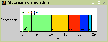
This algorithm solves
1|rj|Cmax scheduling problem.
Tha basic idea of the algorithm is to arrange and schedule the tasks in
order of nondecreasing release time
rj. It is equivalent to the
First Come First Served rule (FCFS). The algorithm usage is outlined in
Figure 7.1 and the correspondin
schedule is displayed in Figure
7.2 as a Gantt chart.
TS = alg1rjcmax(T,problem)
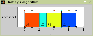
Bratley’s algorithm, proposed to solve
1|rj,~dj|Cmax
problem, is algorithm which uses branch and bound method. Problem is from
class NP-hard and finding best solution is based on backtracking in the
tree of all solutions. Number of solutions is reduced by testing
availabilty of schedule after adding each task. For more details about
Bratley’s algorithm see [Błażewicz01].
In Figure 7.3 the algorithm usage is shown. The resulting schedule is shown in Figure 7.4.
TS = bratley(T,problem)
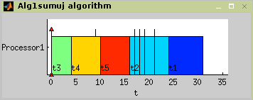
Hodgson's algorithm is proposed to solve 1||ΣUj problem, that means it minimalize number of delayed tasks. Algorithm operates in two steps:
The subset Ts of taskset T, that can be processed on time, is determined.
A schedule is determined from the subsets Ts and Tn = T – Ts (tasks, that can not be processed on time).
Implementation: Apply EDD (Earliest Due Date First) rule on taskset T. If each task can be processed on time, then this is the final schedule. Else move as much tasks with the longest processing time from Ts to Tn as is needed to process each task from Ts on time. Then schedule subset Tn in an arbitrary order. Final schedule is [Ts Tn]. For more details about Hodgson's algorithm see [Błażewicz01].
In Figure 7.5 the algorithm usage is outlined. The resulting schedule is displayed in Figure 7.6.
TS = alg1sumuj(T,problem)
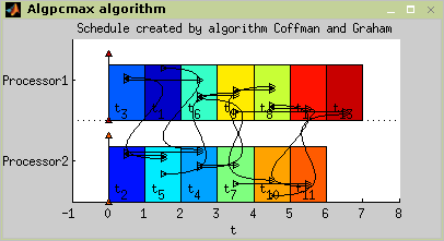
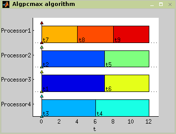
This algorithm solves problem P||Cmax, where a set of independent tasks has to be assigned to parallel identical processors in order to minimize schedule length. Preemption is not allowed. Algorithm finds optimal schedule using Integer Linear Programming (ILP). The algorithm usage is outlined in Figure 7.7 and resulting schedule is displayed in Figure 7.8.
TS = algpcmax(T,problem,processors)
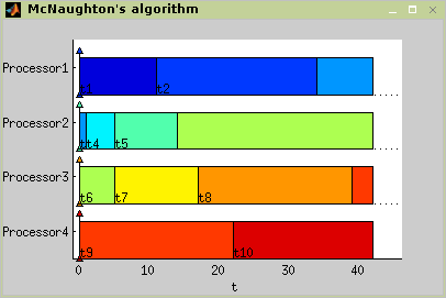
McNaughton’s algorithm solves problem P|pmtn|Cmax, where a set of
independent tasks has to be scheduled on identical processors in order to
minimize schedule length. This algorithm consider preemption of the task
and the resulting schedule is optimal. The maximum length of task schedule
can be defined as maximum of this two values:
max(pj);
(∑pj)/m, where m means number of
processors. For more details about Hodgson’s algorithm see [Błażewicz01].
The algorithm use is outlined in Figure 7.9. The resulting Gantt chart is shown in Figure 7.10.
TS = mcnaughtonrule(T,problem,processors)
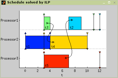
This algorithm is designed for solving
P|rj,prec,~dj|Cmax
problem. The algorithm uses modified List Scheduling algorithm List Scheduling to determine an upper bound of the
criterion Cmax. The optimal schedule is found using ILP(integer linear
programming).
In Figure 7.11 the algorithm usage is shown. The resulting Gantt chart is displayed in Figure 7.12.
TS = algprjdeadlinepreccmax(T,problem,processors)
>> t1 = task('t1',4,0,4);
>> t2 = task('t2',2,3,12);
>> t3 = task('t3',1,3,11);
>> t4 = task('t4',6,3,10);
>> t5 = task('t5',4,3,12);
>> prec = [0 0 0 0 0;...
           0 0 0 0 0;...
           0 0 0 1 0;...
           0 0 0 0 0;...
           0 1 0 0 0];
>> T = taskset([t1 t2 t3 t4 t5],prec);
>> prob = problem('P|rj,prec,~dj|Cmax');
>> TS = algprjdeadlinepreccmax(T,prob,3);
>> plot(TS);
Figure 7.12. Scheduling problem
P|pj,prec,~dj|Cmax
solving.
List Scheduling (LS) is a heuristic algorithm in which tasks are taken from a pre-specified list. Whenever a machine becomes idle, the first available task on the list is scheduled and consequently removed from the list. The availability of a task means that the task has been released. If there are precedence constraints, all its predecessors have already been processed. [Leung04] The algorithm terminates when all the tasks from the list are scheduled. In multiprocessor case, the processor with minimal actual time is taken in each iteration of the algorithm.
Heuristic (suboptimal) algorithms do not guarantee finding the
optimal. A subset of heuristic algorithms constitute approximation
algorithms . It is a group of heuristic algorithms with analytically
evaluated accuracy. The accuracy is measured by absolute
performance ratio. For example when the objective of scheduling
is to minimize Cmax , absolute
performance ratio is defined as  , where
Cmax(A(I)) is
Cmaxobtained by approximation
algorithm A,
Cmax(OPT(I)) is
Cmaxobtained by an optimal
algorithm [Błażewicz01] and Π is a
set of all instances of the given scheduling problem. For an arbitrary List
Scheduling algorithm is proved that
RLS=2-1/m,
where m is the number of processors. Time complexity of
the LS algorithm is O(n).
List Scheduling algorithm is implemented in Scheduling Toolbox as function:
TS = listsch(T,problem,processors [,strategy])
TS = listsch(T,problem,processors [,schoptions])
- T
set of tasks
- problem
object problem
- processors
number of processors
- strategy
strategy for LS algorithm
- schoptions
optimization options (see Section Scheduling Toolbox Options)
The algorithm is able to solve R|prec|Cmax or any easier problem. For more details about List Scheduling algorithm see [Błażewicz01].
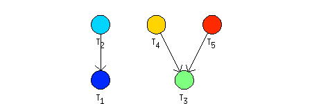
The set of tasks contains five tasks named {`t1', `t2', `t3', `t4', `t5'} with processing times [2 3 1 2 4]. The tasks are constrained by precedence constraints as shown in Figure 7.14, “An example of P|prec|Cmax scheduling problem.”.
Example 7.1. List Scheduling - problem P|prec|Cmax.
>> t1=task('t1',2);
>> t2=task('t2',3);
>> t3=task('t3',1);
>> t4=task('t4',2);
>> t5=task('t5',4);

>> prec = [0 0 0 0 0;...
           1 0 0 0 0;...
           0 0 0 0 0;...
           0 0 1 0 0;...
           0 0 1 0 0];

>> T = taskset([t1 t2 t3 t4 t5],prec);
>> p = problem('P|prec|Cmax');
>> TS = listsch(T,p,2);
>> plot(TS);
Figure 7.15. Scheduling problem P|prec|Cmax solving.
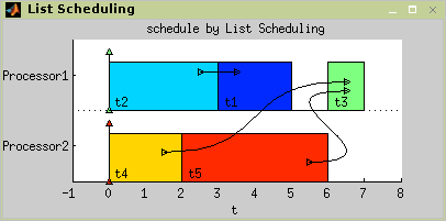
The solution of the example is shown in Figure 7.16, “Result of List Scheduling.”. The LS algorithm found a schedule with
Cmax= 7.
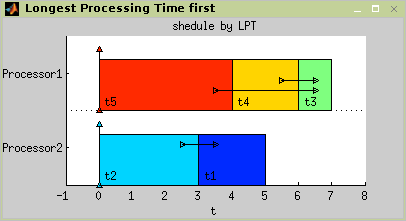
Longest Processing Time first (LPT), intended to solve P||Cmax
problem, is a strategy for LS algorithm in which the tasks are arranged in
order of non increasing processing time
pj before the application of
List Scheduling algorithm. The time complexity of LPT is  . The absolute performance ratio of LPT for
problem P||Cmax is [Błażewicz01.]
. The absolute performance ratio of LPT for
problem P||Cmax is [Błażewicz01.]
LPT is implemented as optional parameter of List Scheduling algorithm and it is able to solve R|prec|Cmax or any easier problem.
RS = listsch(T,problem,processors,'LPT')
LS algorithm with LPT strategy demonstrated on the example from
previous paragraph is shown in Figure 7.17, “Problem P|prec|Cmax by LS algorithm with LPT strategy
solving.”.
The resulting schedule with
Cmax= 7 is in
Figure 7.18, “Result of LS algorithm with LPT strategy.”.
>> t1=task('t1',2);
>> t2=task('t2',3);
>> t3=task('t3',1);
>> t4=task('t4',2);
>> t5=task('t5',4);

>> prec = [0 0 0 0 0;...
           1 0 0 0 0;...
           0 0 0 0 0;...
           0 0 1 0 0;...
           0 0 1 0 0];

>> T = taskset([t1 t2 t3 t4 t5],prec);
>> p = problem('P|prec|Cmax');
>> TS = listsch(T,p,2,'LPT');
>> plot(TS);
Figure 7.17. Problem P|prec|Cmax by LS algorithm with LPT strategy solving.
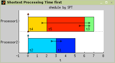
Shortest Processing Time first (SPT), intended to solve P||Cmax
problem, is a strategy for LS algorithm in which the tasks are arranged in
order of nondecreasing processing time
pj before the application of
List Scheduling algorithm. The time complexity of SPT is also  [Błażewicz01.]
SPT is implemented as optional parameter of List Scheduling algorithm and it is able to solve R|prec|Cmax or any easier problem .
TS = listsch(T,problem,processors,'SPT')
LS algorithm with SPT strategy demonstrated on the example from
Figure 7.14, “An example of P|prec|Cmax scheduling problem.” is shown in Figure 7.19, “Solving P|prec|Cmax by LS algorithm with SPT strategy.”. The resulting schedule with
Cmax= 7 is in
Figure 7.20, “Result of LS algorithm with SPT strategy.”.
>> t1=task('t1',2);
>> t2=task('t2',3);
>> t3=task('t3',1);
>> t4=task('t4',2);
>> t5=task('t5',4);

>> prec = [0 0 0 0 0;...
           1 0 0 0 0;...
           0 0 0 0 0;...
           0 0 1 0 0;...
           0 0 1 0 0];

>> T = taskset([t1 t2 t3 t4 t5],prec);
>> p = problem('P|prec|Cmax');
>> TS = listsch(T,p,2,'SPT');
>> plot(TS);
Figure 7.19. Solving P|prec|Cmax by LS algorithm with SPT strategy.
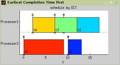
Earliest Completion Time first (ECT), intended to solve P||∑Cj
problem, is a strategy for LS algorithm in which the tasks are arranged in
order of nondecreasing completion time
Cj in each iteration of List
Scheduling algorithm. The time complexity of ECT is equal or better than
 .
.
ECT is implemented as optional parameter of List Scheduling algorithm and it is able to solve R|rj, prec|∑wjCj or any easier problem.
TS = listsch(T,problem,processors,'ECT')
An example of P|rj|∑wjCj scheduling problem given with set of five
tasks with names, processing time and release time is shown in Table 7.2, “An example of P|rj|∑wjCj scheduling problem.”. The schedule obtained by ECT strategy
with ∑Cj = 58 is shown in Figure 7.24, “Result of LS algorithm with EST strategy.”.
| name | processing time | release time |
| t1 | 3 | 10 |
| t2 | 5 | 9 |
| t3 | 5 | 7 |
| t4 | 5 | 2 |
| t5 | 9 | 0 |
Table 7.2. An example of P|rj|∑wjCj scheduling problem.
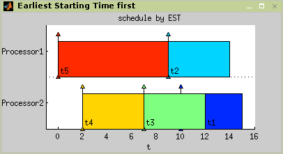
Earliest Starting Time first (EST), intended to solve P||∑Cj
problem, is a strategy for LS algorithm in which the tasks are arranged in
order of nondecreasing starting time
rj before the application of
List Scheduling algorithm. The time complexity of EST is  .
.
EST is implemented as an optional parameter to List Scheduling algorithm and it is able to solve R|rj, prec|∑wjCj or any easier problem.
TS = listsch(T,problem,processors,'EST')
LS algorithm with EST strategy demonstrated on the example from
Figure 7.14, “An example of P|prec|Cmax scheduling problem.” is shown in Figure 7.23, “Problem P|rj|∑Cj by LS algorithm with EST strategy
solving.”. The resulting schedule with
∑Cj = 57 is in Figure 7.24, “Result of LS algorithm with EST strategy.”.
It's possible to define own strategy for LS algorithm according to the following model of function. Function with the same name as the optional parameter (name of strategy function) is called from List Scheduling algorithm:
TS = listsch(T,problem,processors,'OwnStrategy')
In this case, strategy algorithm is called in each iteration of List Scheduling algorithm upon the set of unscheduled task. Strategy algorithm is a standalone function with following parameters:
[TS, order] = OwnStrategy(T[,iteration,processor]);
- T
set of tasks
- order
index vector representing new order of tasks
- iteration
actual iteration of List Scheduling algorithm
- processor
selected processor
The internal structure of the function can be similar to implementation of EST strategy in private directory of scheduling toolbox.
function [TS, order] = OwnStrategy(T, varargin) % head

% body
if nargin>1
    if varargin{1}>1
        order = 1:length(T.tasks);
        return
    end
end

wreltime = T.releasetime./taskset.weight;
[TS order] = sort(T,wreltime,'inc'); % sort taskset
% end of body
Figure 7.25. An example of OwnStrategy function.
Standard variable varargin represents optional
parameters iteration and processor.
The definition of this variable is required in the head of function when
it is used with listsch.
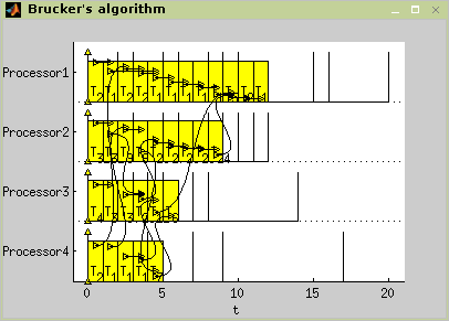
Brucker’s algorithm, proposed to solve
1|in-tree,pj=1|Lmax problem, is
an algorithm which can be implemented in O(n.log n) time [Bru76][, Błażewicz01]. Implementation in the toolbox use
listscheduling algorithm while tasks are sorted in non-increasing order of
theyr modified due dates subject to precedence constraints. The algorithm
returns an optimal schedule with respect to criterion
Lmax. Parameters of the function solving this
scheduling problem are described in the Reference Guide brucker76.m.
Examples in Figure 7.26, “Scheduling problem
1|in-tree,pj=1|Lmax
solving.” and Figure 7.27, “Brucker’s algorithm - problem
1|in-tree,pj=1|Lmax” show, how an instance of the scheduling
problem [Błażewicz01] can be
solved by the Brucker's algorithm. For more details see
brucker76_demo in
\scheduling\stdemos.
Traditional scheduling algorithms (e.g., Błażewicz01) typically assume that deadlines are absolute. However in many real applications release date and deadline of tasks are related to the start time of another tasks [Brucker99][Hanzalek04]. This problem is in literature called scheduling with positive and negative time-lags.
The scheduling problem is given by a task-on-node graph
G. Each task
ti is represented by node
ti in graph G and has a positive
processing time pi. Timing
constraints between two nodes are represented by a set of directed edges.
Each edge eij from the node
ti to the node
tj is labeled with an integer
time lag wij. There are two
kinds of edges: the forward edges with positive time
lags and the backward edges with negative time lags.
The forward edge from the node ti to the node
tj with the positive time lag
wij indicates that
sj, the start time of
tj, must be at least
wij time units after
si, the start time of
ti. The backward edge from node
tj to node
ti with the negative time lag
wji indicates that
sj must be no more than
wji time units after
si. The objective is to find a
schedule with minimal
Cmax.
Since the scheduling problem is NP-hard [Brucker99], algorithm implemented in the toolbox is based on branch and bound algorithm. Alternative implemented solution uses Integer Linear Programming (ILP). The algorithm call has the following syntax:
TS = spntl(T,problem,schoptions)
- problem
an object of type problem describing the classification of deterministic scheduling problems (see Section Chapter 5, Classification in Scheduling). In this case the problem with positive and negative time lags is identified by `SPNTL'.
- schoptions
optimization options (see Section Scheduling Toolbox Options)
The algorithm can be chosen by the value of parameter
schoptions - structure schoptions
(see Scheduling Toolbox Options). For more
details on algorithms please see [Hanzalek04].
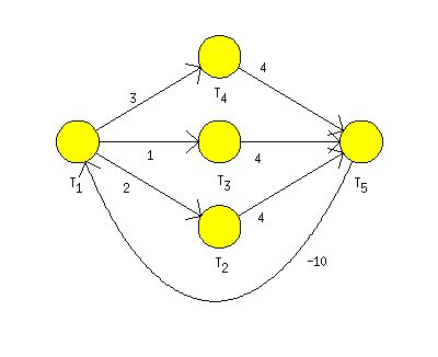
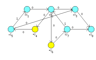
An example of the scheduling problem containing five tasks is
shown in Figure 7.28, “Graph G representing tasks constrained by
positive and negative time-lags.” by graph
G. Execution times are
p=(1,3,2,4,5) and delay between start times of tasks
t1 and
t5 have to be less then or
equal to 10
(w5,1=-10).
The objective is to find a schedule with minimal
Cmax.
Example 7.2. Example of Scheduling Problem with Positive and Negative Time-Lags.
Solution of this scheduling problem using spntl
function is shown below. Graph of the example can be found in Scheduling
Toolbox directory <Matlab
root>\toolbox\scheduling\stdemos\benchmarks\spntl\spntl_graph.matG corresponding to the example shown in Figure 7.28, “Graph G representing tasks constrained by
positive and negative time-lags.” can be opened and edited in Graphedit tool
(graphedit(g)).
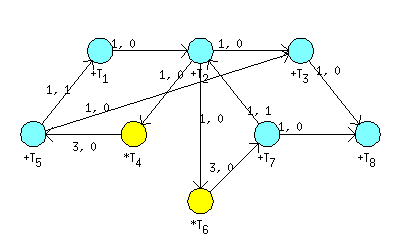
Resulting graph G is shown in Figure 7.31, “Graph G weighted by
lij and
hij of WDF.”. Finaly, the graph
G is used to generate an object taskset describing the
scheduling problem. Parameters conversion must be specified as parameters
of function taskset. For example in our case, the
function is called with following parameters:
T = taskset(LHgraph,'n2t',@node2task,'ProcTime','Processor', ...
       'e2p',@edges2param)
For more details see Section 5, “Transformations Between Objects taskset and
graph”. The optimal solution in Figure 7.29, “Resulting schedule of instance in Figure 7.28, “Graph G representing tasks constrained by
positive and negative time-lags.”.” was obtained in the toolbox as is depicted
below.
>> load <Matlab root>\toolbox\scheduling\stdemos\benchmarks\spntl_graph
>> graphedit(g)
>> T = taskset(LHgraph,'n2t',@node2task,'ProcTime','Processor', ...
       'e2p',@edges2param)
Set of 5 tasks
 There are precedence constraints
>> prob=problem('SPNTL')
SPNTL
>> schoptions=schoptionsset('spntlMethod','BaB');
>> T = spntl(T, prob, schoptions)
Set of 5 tasks
 There are precedence constraints
 There is schedule: SPNTL - BaB algorithm
>> plot(t)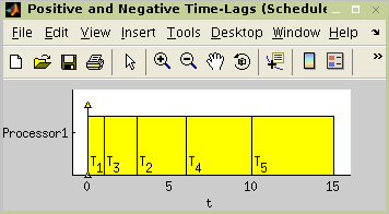
Figure 7.29. Resulting schedule of instance in Figure 7.28, “Graph G representing tasks constrained by
positive and negative time-lags.”.
Many activities e.g. in automated manufacturing or parallel computing are cyclic operations. It means that tasks are cyclically repeated on machines. One repetition is usually called an iteration and common objective is to find a schedule that maximises throughput. Many scheduling techniques leads to overlapped schedule, where operations belonging to different iterations can execute simultaneously.
Cyclic scheduling deals with a set of
operations (generic tasks ti) that have to be
performed infinitely often [Hanen95]. Data dependencies of this problem can
be modeled by a directed graph G. Each task
ti is represented by the node
ti in the graph
G and has a positive processing time
pi. Edge
eij from the node
ti to tj is labeled by a
couple of integer constants lij
and hij. Length
lij represents the minimal
distance in clock cycles from the start time of the task
ti to the start time of
tj and it is always greater than
zero. On the other hand, the height
hij specifies the shift of the
iteration index (dependence distance) from task
ti to task
tj.
Assuming periodic schedule with
period w, i.e. the constant
repetition time of each task, the aim of the cyclic scheduling problem
[Hanen95] is to find a periodic
schedule with minimal period w. In modulo scheduling
terminology, period w is called Initiation Interval
(II).
The algorithm available in this version of the toolbox is based on
work presented in [Hanzalek07] and [Sucha07]. Function
cycsch solves cyclic scheduling of tasks with
precedence delays on dedicated sets of parallel identical processors. The
algorithm uses Integer Linear Programming
TS = cycsch(T,problem,m,schoptions)
- problem
object of type problem describing the classification of deterministic scheduling problems (see Section Chapter 5, Classification in Scheduling). In this case the problem is identified by `CSCH'.
- m
vector with number of processors in corresponding groups of processors
- schoptions
optimization options (see Section Scheduling Toolbox Options)
In addition, the algorithm minimizes the iteration overlap
[Sucha04]. This
secondary objective of optimization can be disabled in parameter
schoptions, i.e. parameter
secondaryObjective of schoptions
structure (see Scheduling Toolbox Options). The
optimization option also allows to choose a method for Cyclic Scheduling
algorithm, specify another ILP solver, enable/disable elimination of
redundant binary decision variables and specify another ILP solver for
elimination of redundant binary decision variables.
For more details on the algorithm please see [Sucha04].
An example of an iterative algorithm used in Digital Signal Processing as a benchmark is Wave Digital Filter (WDF) Fettweis86.
for k=1 to N do
   a(k) =X(k) + e(k-1)  %T1
   b(k) = a(k) - g(k-1) %T2
   c(k) = b(k) + e(k)   %T3
   d(k) = gamma1 * b(k) %T4
   e(k) = d(k) + e(k-1) %T5
   f(k) = gamma2 * b(k) %T6
   g(k) = f(k) + g(k-1) %T7
   Y(k) = c(k) - g(k)   %T8
end
The corresponding Cyclic Data Flow Graph is shown in Figure 7.30, “Cyclic Data Flow Graph of WDF.”. Constant on nodes indicates the
number of dedicated group of processors. The objective is to find a
cyclic schedule with minimal period w on one add and
one mul unit. Input-output latency of add (mul) unit is 1 (3) clock
cycle(s).
Example 7.3. Cyclic Scheduling - Wave Digital Filter.
To transform Cyclic Data Flow Graph (CDFG) to graph
G weighted by
lij and
hij function LHgraph can be
used:
LHgraph = cdfg2LHgraph(dfg,UnitProcTime,UnitLattency)
- LHgraph
graph
Gweighted bylij andhij- dfg
Data Flow Graph where user parameter (UserParam) on nodes represents dedicated processor and user parameter (UserParam) on edges correspond to dependence distance - height of the edge.
- UnitProcTime
vector of processing time of tasks on dedicated processors
- UnitLattency
vector of input-output latency of dedicated processors
Resulting graph G is shown in Figure 7.31, “Graph G weighted by
lij and
hij of WDF.”. Finaly, the graph
G is used to generate an object taskset describing the
scheduling problem. Parameters conversion must be specified as parameters
of function taskset. For example in our case, the
function is called with following parameters:
T = taskset(LHgraph,'n2t',@node2task,'ProcTime','Processor', ...
       'e2p',@edges2param)
For more details see Section 5, “Transformations Between Objects taskset and
graph”.
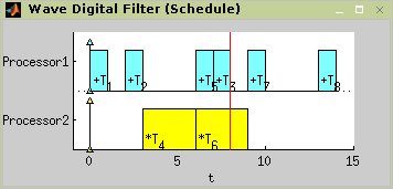
The scheduling procedure (shown below) found schedule depicted in
Figure 7.32, “Resulting schedule with optimal period
w=8.”.
>> load <Matlab root>\toolbox\scheduling\stdemos\benchmarks\dsp\wdf
>> graphedit(wdf)
>> UnitProcTime = [1 3];
>> UnitLattency = [1 3];
>> m = [1 1];
>> LHgraph = cdfg2LHgraph(wdf,UnitProcTime,UnitLattency)

 adjacency matrix:
     0     1     0     0     0     0     0     0
     0     0     1     0     0     0     1     1
     0     0     0     1     0     0     0     0
     0     0     0     0     0     0     0     0
     0     1     0     1     0     0     0     0
     1     0     1     0     0     0     0     0
     0     0     0     0     0     1     0     0
     0     0     0     0     1     0     0     0
>>
>> graphedit(LHgraph)
>> T = taskset(LHgraph,'n2t',@node2task,'ProcTime','Processor', ...
       'e2p',@edges2param)
Set of 8 tasks
 There are precedence constraints
>> prob = problem('CSCH');
>> schoptions = schoptionsset('ilpSolver','glpk', ...
'cycSchMethod','integer','varElim',1);
>> TS = cycsch(T, prob, m, schoptions)
Set of 8 tasks
 There are precedence constraints
 There is schedule: General cyclic scheduling algorithm (method:integer)
   Tasks period: 8
   Solving time: 1.113s
   Number of iterations: 4
>> plot(TS,'prec',0)
Graph of WDF benchmark [Fettweis86] can be found in Scheduling Toolbox
directory <Matlab
root>\toolbox\scheduling\stdemos\benchmarks\dsp\wdf.mat
This section presents the SAT based approach to the scheduling problems. The main idea is to formulate a given scheduling problem in the form of CNF (conjunctive normal form) clauses. TORSCHE includes the SAT based algorithm for P|prec|Cmax problem.
Before use you have to instal SAT solver.
Download the zChaff SAT solver (version: 2004.11.15) from the zChaff web site.
Place the dowloaded file zchaff.2004.11.15.zip to the
<TORSCHE>\contribfolder.Be sure that you have C++ compiler set to the mex files compiling. To set C++ compiler call:
>> mex -setup
For Windows we tested Microsoft Visual C++ compiler, version 7 and 8. (Version 6 isn't supported.)
For Linux use gcc compiler.
From Matlab workspace call m-file
make.min<TORSCHE>\satfolder.
In the case of P|prec|Cmax problem, each CNF clause is a function
of Boolean variables in the form  . If task ti is started at
time unit
. If task ti is started at
time unit j on the processor k
then  , otherwise . For each task
ti, where  , there are
  Boolean variables, where
 S
denotes the maximum number of time units and R
denotes the total number of processors.
The Boolean variables are constrained by the three following rules (modest adaptation of [Memik02]):
For each task, exactly one of the
variables has to be equal to 1. Therefore two
clauses are generated for each task ti. The
first guarantees having at most one variable equal to 1 (true):
 The second guarantees having at least one
variable equal to 1:
The second guarantees having at least one
variable equal to 1: 
If there is a precedence constrains such that tu is the predecessor of
tv, thentv cannot start before the execution oftu is finished. Therefore, for all possible combinations of processors
kandl, wherepu denotes the processing time of tasktu.At any time unit, there is at most one task executed on a given processor. For the couple of tasks with a precedence constrain this rule is ensured already by the clauses in the rule number 2. Otherwise the set of clauses is generated for each processor
kand each time unitjfor all couplestu,tv without precedence constrains in the following form:
In the toolbox we use a zChaff solver to
decide whether the set of clauses is satisfiable. If it is, the schedule
within S time units is feasible. An optimal schedule
is found in iterative manner. First, the List Scheduling algorithm is
used to find initial value of S. Then we iteratively
decrement value of S by one and test feasibility of
the solution. The iterative algorithm finishes when the solution is not
feasible.
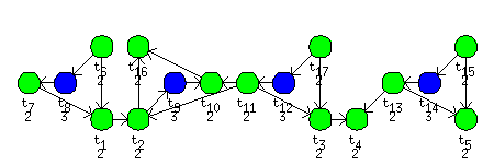
As an example we show a computation loop of a Jaumann wave digital
filter. Our goal is to minimize computation time of the filter loop,
shown as directed acyclic graph in Figure 7.33, “Jaumann wave digital filter”.
Nodes in the graph represent the tasks and the edges represent
precedence constraints. Green nodes represent addition operations and
blue nodes represent multiplication operations. Nodes are labeled by the
processing time pi. We look
for an optimal schedule on two parallel identical processors.
Folowing code shows consecutive steps performed within the
toolbox. First, we define the set of task with precedence constrains and
then we run the scheduling algorithm satsch.
Finally we plot the Gantt chart.
>> procTime = [2,2,2,2,2,2,2,3,3,2,2,3,2,3,2,2,2];
>> prec = sparse(...
[6,7,1,11,11,17,3,13,13,15,8,6,2,9 ,11,12,17,14,15,2 ,10],...
[1,1,2,2 ,3 ,3 ,4,4 ,5 ,5 ,7,8,9,10,10,11,12,13,14,16,16],...
[1,1,1,1 ,1 ,1 ,1,1 ,1 ,1 ,1,1,1,1 ,1 ,1 ,1 ,1 ,1 ,1 ,1],...
17,17);
>> jaumann = taskset(procTime,prec);
>> jaumannSchedule = satsch(jaumann,problem('P|prec|Cmax'),2)
Set of 17 tasks
There are precedence constraints
There is schedule: SAT solver
SUM solving time: 0.06s
MAX solving time: 0.04s
Number of iterations: 2
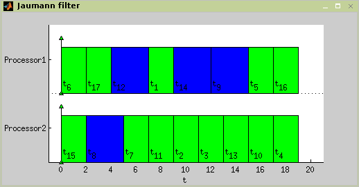
>> plot(jaumannSchedule)The satsch algorithm performed two
iterations. In the first iteration 3633 clauses with 180 variables were
solved as satisfiable for S=19 time units. In the
second iteration 2610 clauses with 146 variables were solved with
unsatisfiable result for S=18 time units. The optimal
schedule is depicted in Figure 7.34, “The optimal schedule of Jaumann filter”.
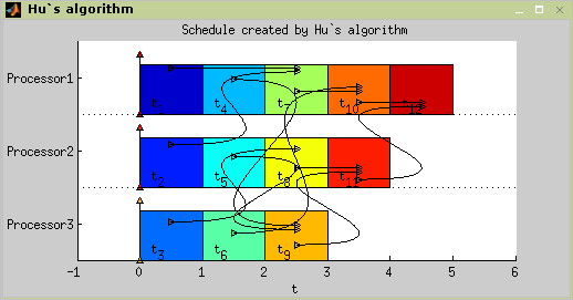
Hu's algorithm is intend to schedule unit length tasks with in-tree
precedence constraints. Problem notatin is
P|in-tree,pj=1|Cmax. The
algorithm is based on notation of in-tree levels, where in-tree level is
number of tasks on path to the root of in-tree graph. The time complexity
is O(n).
TS = hu(T,problem,processors[,verbose])
or
TS = hu(T,problem,processors[,schoptions])
- verbose
level of verbosity
- schoptions
optimization options
For more details about Hu's algorithm see [Błażewicz01].
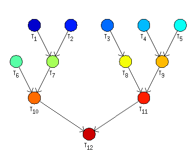
There are 12 unit length tasks with precedence constraints defined as in Figure 7.35, “An example of in-tree precedence constraints”.
Example 7.4. Hu's algorithm
>> t1=task('t1',1);
>> t2=task('t2',1);
>> t3=task('t3',1);
>> t4=task('t4',1);
>> t5=task('t5',1);
>> t6=task('t6',1);
>> t7=task('t7',1);
>> t8=task('t8',1);
>> t9=task('t9',1);
>> t10=task('t10',1);
>> t11=task('t11',1);
>> t12=task('t12',1);

>> p = problem('P|in-tree,pj=1|Cmax');
>> prec = [
    0 0 0 0 0 0 1 0 0 0 0 0
    0 0 0 0 0 0 1 0 0 0 0 0
    0 0 0 0 0 0 0 1 0 0 0 0
    0 0 0 0 0 0 0 0 1 0 0 0
    0 0 0 0 0 0 0 0 1 0 0 0
    0 0 0 0 0 0 0 0 0 1 0 0
    0 0 0 0 0 0 0 0 0 1 0 0
    0 0 0 0 0 0 0 0 0 0 1 0
    0 0 0 0 0 0 0 0 0 0 1 0
    0 0 0 0 0 0 0 0 0 0 0 1
    0 0 0 0 0 0 0 0 0 0 0 1
    0 0 0 0 0 0 0 0 0 0 0 0
    ];
>> T = taskset([t1 t2 t3 t4 t5 t6 t7 t8 t9 t10 t11 t12],prec);

>> TS= hu(T,p,3);
>> plot(TS);
Figure 7.36. Scheduling problem
P|in-tree,pj=1|Cmax using
hu command
This algorithm generate optimal solution for
P2|prec,pj=1|Cmax problem. Unit
length tasks are scheduled nonpreemptively on two processors with time
complexity O(n2). Each task
is assigned by label, which take into account the levels and the numbers
of its imediate successors. Algorithm operates in two steps:
Assign labels to tasks.
Schedule by Hu's algorithm, use labels instead of levels.
TS = coffmangraham(T,problem[,verbose])
or
TS = coffmangraham(T,problem[,schoptions])
- schoptions
optimization options
More about Coffman and Graham algorithm in [Błażewicz01].
The set of tasks contains 13 tasks constrained by precedence constraints as shown in Figure 7.38, “Coffman and Graham example setting”.
Example 7.5. Coffman and Graham algorithm
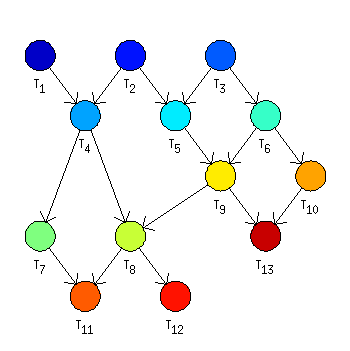
>> t1 = task('t1',1);
>> t2 = task('t2',1);
>> t3 = task('t3',1);
>> t4 = task('t4',1);
>> t5 = task('t5',1);
>> t6 = task('t6',1);
>> t7 = task('t7',1);
>> t8 = task('t8',1);
>> t9 = task('t9',1);
>> t10 = task('t10',1);
>> t11 = task('t11',1);
>> t12 = task('t12',1);
>> t13 = task('t13',1);
>> t14 = task('t14',1);

>> p = problem('P2|prec,pj=1|Cmax');
>> prec = [
        0 0 0 1 0 0 0 0 0 0 0 0 0
        0 0 0 1 1 0 0 0 0 0 0 0 0
        0 0 0 0 1 1 0 0 0 0 0 0 0
        0 0 0 0 0 0 1 1 0 0 0 0 0
        0 0 0 0 0 0 0 0 1 0 0 0 0
        0 0 0 0 0 0 0 0 1 1 0 0 0
        0 0 0 0 0 0 0 0 0 0 1 0 0
        0 0 0 0 0 0 0 0 0 0 1 1 0
        0 0 0 0 0 0 0 1 0 0 0 0 1
        0 0 0 0 0 0 0 0 0 0 0 0 1
        0 0 0 0 0 0 0 0 0 0 0 0 0
        0 0 0 0 0 0 0 0 0 0 0 0 0
        0 0 0 0 0 0 0 0 0 0 0 0 0
    ];
>> T = taskset([t1 t2 t3 t4 t5 t6 t7 t8 t9 t10 t11 t12 t13 t14],prec);

>> TS= coffmangraham(T,p);
>> plot(TS);