TORSCHE Scheduling
Toolbox for Matlab

TORSCHE Scheduling Toolbox for Matlab (0.4.0) currently supports MATLAB 6.5 (R13) and higher versions. If you want to use the toolbox on different platforms than MS-Windows or Linux on PC (32bit) compatible, some algorithms must be compiled by a C/C++ compiler. We recommend to use Microsoft Visual C/C++ 7.0 and higher under Windows or gcc under Linux.

Download the toolbox from web and unpack Scheduling toolbox into the directory where Matlab toolboxes are installed (most often in <Matlab root>\toolbox on Windows systems and on Linux systems in <Matlab root>/toolbox). Run Matlab and add two new paths into directories with Scheduling toolbox and demos, e.g.:

>> addpath(path,'c:\matlab\toolbox\scheduling')
>> addpath(path,'c:\matlab\toolbox\scheduling\stdemos')

Several algorithms in the toolbox are implemented as Matlab MEX-files (compiled C/C++ files). Compiled MEX-files for MS-Windows and Linux on PC (32bit) compatible are part of this distribution. If you use the toolbox on a different platform, please compile these algorithms using command make from \scheduling directory (in Matlab environment). Before that, please specify the compiler using command mex -setup from (also in Matlab environment). We suggest to use Microsoft Visual C/C++ or gcc compilers.

To display a list of all available commands and functions please type

>> help scheduling

To get help on any of the toolbox commands (e.g. task) type

>> help task

To get help on overloaded commands, i.e. commands that do exist somewhere in Matlab path (e.g. plot) type

>> help task/plot

Or alternatively type help plot and then select task/plot at the bottom line line of the help text.

Solving procedure of your scheduling problem can be divided into four basic steps:

Task is defined by command task, for example:

>> t1 = task('task1', 5, 1, inf, 12)
Task "task1"
 Processing time: 5
 Release time:    1
 Due date:        12

This command defines task with name ``task1", processing time 5, release time 1, and duedate at time 12. In the same way we can define next tasks:

>> t2 = task('task2', 2, 0, inf, 11);
>> t3 = task('task3', 3, 5, inf, 9);

To create a set of tasks use command taskset:

>> T = taskset([t1 t2 t3])
Set of 3 tasks

For short:

>> T = [t1 t2 t3]
Set of 3 tasks

Due to great variety of scheduling problems, it is not easy to choose a proper algorithm. For easier selection of the proper algorithm, the toolbox uses a notation, proposed by [Graham79] and [Błażewicz83], to classify scheduling problems. Those classifications are created by command problem:

>> p=problem('1|pmtn,rj|Lmax')
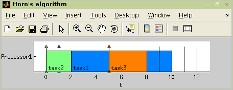
1|pmtn,rj|Lmax

Now we can execute the scheduling algorithm, for example Horn's algorithm:

>> TS = horn(T,p)
Set of 3 tasks
 There is schedule: Horn's algorithm
   Solving time: 0.29s

The final schedule, given by Gantt chart ,is shown in Figure 2.1, “The taskset schedule”. The figure is plotted by:

>> plot(TS)

Figure 2.1. The taskset schedule

Data from the Matlab workspace can be saved and loaded by standard commands save and load. For example:

>> save file1
>> save file2 t1 t2

>> load file2