TORSCHE Scheduling
Toolbox for Matlab

TORSCHE – Sets of Tasks

Table of Contents

1. Creating the taskset Object
2. Graphical Representation of the Set of Tasks
3. Set of Tasks Modification
4. Other Functions

1. Creating the `taskset` Object

Objects of the type task can be grouped into a set of tasks. A set of tasks is an object of the type taskset which can be created by the command taskset. Syntax for this command is:

T = taskset(tasks[,prec])

where variable tasks is an array of objects of the type task. Furthermore, relations between tasks can be defined by precedence constraints in parameter prec. Parameter prec is an adjacency matrix (see Chapter 6, Graphs) defining a graph where nodes correspond to tasks and edges are precedence constraints between these tasks. If there is an edge from T_i to T_j in the graph, it means that T_i must be completed before T_j can be started.

If there are not precedence constraints between the tasks, we can use a shorter form of creating a set of tasks using square brackets (see the first line in Figure 4.1, “Creating a set of tasks and adding precedence constraints”).

>> T1 = [t1 t2 t3]
Set of 3 tasks

>> T1 = taskset(T1,[0 1 1; 0 0 1; 0 0 0])
Set of 3 tasks
 There are precedence constraints
 
>> T2 = taskset([3 4 2 4 4 2 5 4 8])
Set of 9 tasks

Figure 4.1. Creating a set of tasks and adding precedence constraints

You can also create a set of tasks directly from a vector of processing times. Call the command taskset as shown in Figure 4.1, “Creating a set of tasks and adding precedence constraints”. Tasks with those processing times will be automatically created inside the set of tasks. Precedence constraints can be added in the same way as in case of taskset T1 (see Figure 4.1, “Creating a set of tasks and adding precedence constraints”).

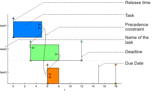
2. Graphical Representation of the Set of Tasks

As for single tasks, command plot can be used to draw parameters of set of tasks graphically. An example of plot output with explanation of used marks is shown in Figure 4.2, “Gantt chart for a set of scheduled tasks”. For more details see Reference Guide @taskset/plot.m.

>> plot(T1)

Figure 4.2. Gantt chart for a set of scheduled tasks

3. Set of Tasks Modification

Commands changing parameters of tasksets are the same as for task object. Command get returns the value of the specified property or values of all properties. Command set sets the value of the specified property. These two commands has got a standard syntax, which is described in Matlab user manual. Property access is allowed over the . (dot) operator too.

Note

To obtain a list of all accessible properties use command get. Note that some private and virtual properties aren't accessible over the . (dot) operator, although they are displayed when the automatic completion by Tab key is used.

3.1. Modification of Tasks Parameters Inside the Set of Tasks

Tasks parameters may be modified via virtual properties of object taskset. The list of virtual properties are: Name, ProcTime, ReleaseTime, Deadline, DueDate, Weight, Processor, UserParam. All parameters are arrays data type. Items order in the arrays is the same as tasks order in the set of the tasks.

>> T2.ProcTime
ans =
     3     4     2     4     4     2     5     4     8
>> T2.ProcTime(3) = 5;
>> T2.ProcTime
ans =
     3     4     5     4     4     2     5     4     8
>> T2.ProcTime = T2.ProcTime -1;
>> T2.ProcTime
ans =
     2     3     4     3     3     1     4     3     7

Figure 4.3. Access to the virtual property examples

3.2. Schedule

The only way how to operate with schedule of tasks is through commands add_schedule and get_schedule. Command add_schedule inserts a schedule (i.e. start time s_j, number of assigned processor, ...) into taskset object. Its syntax is described in Reference Guide @taskset/add_schedule.m. An example of add_schedule command use is shown in Figure 4.4, “Schedule inserting example”. Vector start is vector of start times (i.e. first task starts at 0), vector processor is vector of assigned processors (i.e. first task is assigned to the firs processor) and string description is a brief note on used scheduling algorithm.

>> start = [0 0 2 3 6 6 7 9 11];
>> processor = [1 2 1 2 1 2 2 1 2];
>> description = 'a handmade schedule';
>> add_schedule(T2,description,start,T2.ProcTime,processor);
>>
>> get_schedule(T2)
ans =
     0     0     2     3     6     6     7     9    11
>> plot(T2);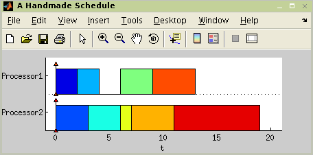

Figure 4.4. Schedule inserting example

On the other hand, the schedule can be obtained from a taskset using command get_schedule (e.g. as is shown in Figure 4.4, “Schedule inserting example”). For more details about this function see Reference Guide @taskset/get_schedule.m. Graphical schedule interpretation (Gantt chart) can be obtained using function plot.

Parameters of a given schedule (e.g. value of optimality criteria, solving time, ...) can be obtained using function schparam. It returns information about schedule inside the taskset and its syntax is described in Reference Guide @taskset/schparam.m. An example of use is shown in Figure 4.5, “Schedule parameters”.

>> param = schparam(T2,'cmax')
param =
    19

>> param = schparam(T2)
param = 
          cmax: 19
         sumcj: 80
        sumwcj: 80

Figure 4.5. Schedule parameters

4. Other Functions

4.1. Count and Size

Commands count(T) and size(T) return number of tasks in the set of tasks T. At this moment they return the same value. Returned value will be different after implementing the general shop problems into the toolbox. Now it is recommended to use command count.

4.2. Sort

The function returns sorted set of tasks inside taskset over selected parameter. Its syntax is described in Reference Guide @taskset/sort.m. An example is shown in Figure 4.6, “Taskset sort example”.

>> T2.ProcTime
ans =
     2     3     4     3     3     1     4     3     7
>> T3 = sort(T2,'ProcTime','dec');
>> T3.ProcTime
ans =
     7     4     4     3     3     3     3     2     1

Figure 4.6. Taskset sort example

4.3. Random taskset

Random taskset T can be created by the command randtaskset. Tasks parameters in the taskset are generated with a uniform distribution. The syntax is described in Reference Guide randtaskset.m. Example of its application is shown in Figure 4.7, “Example of random taskset use”.

>> T = randtaskset(8,[8 15],[3 6]);

>> T.ProcTime
ans =
    15    12    14    11    14    12    14     9

>> T.ReleaseTime
ans =
     4     4     5     3     4     5     5     4

Figure 4.7. Example of random taskset use