Table of Contents
Graphs and graph algorithms are often used in scheduling algorithms, therefore operations with graphs are supported in the toolbox. A graph is data structure including a set of nodes, a set of edges and information on their relations. As it is known from definition of graph from graph theory: G = (V,E,ε). If ε is a binary relation of E over V, then G is called a direct graph. When there is no concern about the direction of an edge, the graph is called undirected. Object Graph in the toolbox is described as directed graph. Undirected graph can be created by addition of another identical edge in opposite direction.
There is a few of different ways of creating a graph because there are several methods how to express it. The object graph is generally described by an adjacency matrix[1]. Graph object is created by the command with the following syntax:
g = graph('adj',A)where variable A is an adjacency matrix. It is
also possible to describe a graph by an incidency matrix[2]. The syntax is:
g = graph('inc',I)where
vaiable I is an incidency matrix. Another way of
creating Graph object is based upon a matrix of edges weights[3]. It is obvious, that just simple graphs can be created by
this way. The syntax in this case is:
g = graph(B)
Any key-word is not required here. This method is considered to be default one because it makes easy setting of weight of an edge. The value of weight is automatically saved as user parameter of the edge. The most complex way of graph creating is definition by a list of edges (or/and nodes). The list of edges (nodes) in the form of cell type is ordered as an argument of the graph function. The cell contains information about initial and terminal node (or number of the node) and arbitrary count of user parameters (e.g. weight of an edge/node). The syntaxe is:
g = graph('edl',edgeList,'ndl',nodeList)where edgeList is list of edges and
nodeList is list of nodes. An example of graphs
creation is shown in Figure 6.1, “Creating a graphs from adjacency matrix”.
>> g1 = graph('adj',[0 2 0; 0 1 0; 0 0 0])

 adjacency matrix:
     0     2     0
     0     1     0
     0     0     0

>> g2 = graph([inf 2; 1 inf])

 adjacency matrix:
     0     1
     1     0

>> g3 = graph('inc',[0 1 0 -1 -1; 1 0 -1 1 1; -1 -1 1 0 0])

 adjacency matrix:
     0     0     1
     2     0     1
     0     1     0

>> g4 = graph('edl',{1,2, 35,[5 8]; 2,3, 68,[2 7]})

 adjacency matrix:
     0     1     0
     0     0     1
     0     0     0
Figure 6.1. Creating a graphs from adjacency matrix
Another possibility to create the object graph is to use a tool
Graphedit, or transform an object taskset to the graph
(see Section 5, “Transformations Between Objects taskset and
graph”).
Command get returns a value of the specified
property or values of all properties. Command set
sets the value of the specified property. These two commands have the same
syntax as is described in Matlab user's guide. Property access is allowed
over the . (dot) operator too.
To obtain list of parameters which can by modified use Command
set, as is shown bellow.
>> set(g2)
                 Name: Name of the GRAPHS
                    N: Array of nodes
                    E: Array of edges
            UserParam: User parameters
            DataTypes: Type of UserParam's data
                Color: Color of area of the GRAPH
             GridFreq: Grid frequency
                Notes: An arbitrary string
                  inc: Incidency matrix
                  adj: Adjacency matrix
                  edl: List of edges (cell)
                  ndl: List of nodes (cell)
edgeUserparamDatatype: Cell of data types of edges' UserParam
nodeUserparamDatatype: Cell of data types of nodes' UserParam
Figure 6.2. Command set for graph
Property Name is a graph name and property
N is an array of node objects. Object node includes all
information about node such as name, user parameters ... Property
E is an array of edge objects where object edge carries
all information about edge. Edge order in array is determined by command
between. This command returns edge indexes for all
edges which interconnect two nodes.
Many algorithms (e.g. for cyclic scheduling in Section 4, “Floyd's Algorithm”) consider an edge-weighted graph, i.e. edges
are weighted by one or more parameters. In object
graph these parameters are stored in user parameters
of corresponding edges. To facilitate access to user parameters, the
toolbox contains two couples of functions for geting/seting data from/to
user parameters.
| function | description |
|---|---|
UserParam = edge2param(g) | Returns user parameters of edges in graph
g as an
n-by-n matrix if the
graph is simple and the value of user parameters is numeric,
cell array otherwise. |
g =
param2edge(g,UserParam) | Adds data in an
n-by-n matrix or cell
array to user parameters of edges in graph
g. |
UserParam = node2param(g) | Returns user parameters of nodes in graph
g as a numeric array or cell array. |
g =
param2node(g,UserParam) | Adds data in a numeric array or cell array to user
parameters of n in graph g. |
Table 6.1. List of functions
In addition, functions edge2param and
param2edge are further extended by optional
parameters. The I-th user parameter can be accessed
using
userParam = edge2param(g,I)
and
g = param2edge(g,userParam,I)
Analogical syntax is valid for functions
node2param and param2node.
If there is not edge between two nodes, the corresponding user
parameter is considered to be Inf. If there are
parallel edges or matrix UserParam does not match with graph
g, the algorithm returns cell array. The different
value indicating that there is not an edge can be defined as a parameter
notEdgeParam.
UserParam = edge2param(g,I,notEdgeParam)
and
g = param2edge(g,UserParam,I,notEdgeParam)
An example of practical usage is shown in example of Critical circuit ratio computation.
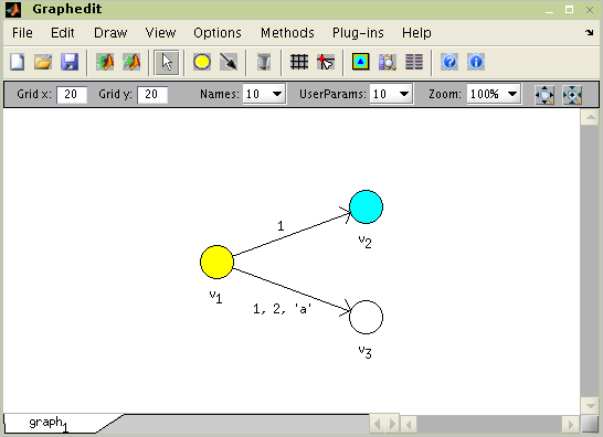
The toolbox is equipped with a simple but useful edi-tor of graphs called Graphedit based on System Handle Graphics of Matlab. It allows construct directed graphs with various user parameters on nodes and edges by simple and intuitive way. The constructed graph can be easily used in the toolbox as instance of object Graph described in the previous subsections, which can be exported to workspace or saved to binary mat-file.
The Graphedit is depicted Figure 6.3, “Graphedit” . As you can see, drawing canvas is the dominant item in the main window. One canvas presents one edited graph. In the bottom of the window are tabs for switching canvases. So there is possibility to work independently with several graphs in one Graphedit. User can find all functions of Graphedit in the main menu. The most used ones are accessible via icons in the toolbar. Properties of graph and its edges and nodes (name, user pa-rameters, color...) may be edited in property editor which is a part of Graphedit.
Graphedit has the following syntax
graphedit(g)
where g is an object graph. To open graphedit
with an empty plot call Graphedit without parameters.
Graphedit operates in four editing modes (Add node, Add edge, Delete and Edit). Selection of mode can be made by four buttons (depicted in Figure 6.3, “Graphedit”) in the toolbar or in main menu. Mode is used for creating and placing of node, mode for connecting nodes by edge, mode for deleting nodes or edges by clicking on it. And properties of nodes and edges can be edited in mode.
Graphedit also offers a possibility to choice appear-ance of a node and contains tool for design your own node-picture which can be formed by bitmapped im-age or any geometric pattern or their arbitrary combi-nation. This function has nothing to do with graph theory; however it is useful for presentation purposes. The system of designing own nodes is displayed in Fig 6.
Placing of nodes or edges is accomplished just by selecting aporiate drawing mode and clicking of the mouse. Each node can be moved by dragging it to a new location. Because the change of shape of edge is often required, every edge is represented by Bézier curves. The way of editing its curve is very similar to way known from common drawing tools dealing with vector graphics. By right click in the edge you display context menu and in it choose 'Edit'. Shape of the edge can be changed by draging little square which has appeared.
Graphedit contains system of plug-ins. It is very helpful tool which allows execution of almost arbitrary function right from GUI of Graphedit via main menu. The function may be some algorithm from toolbox or code implemented by user. The only one condition is, that the function must have object graph as first argument. Other input arguments may be arbitrary; output of the function can be anything – Graph objects will be automatically drown, other data types will be saved into workspace.
By selecting 'Add New Plug-in' in main menu of the Graphedit you can plug in chosen function. Its removing is possible by 'Remove Plugin'.
You can displey Property Editor window by main menu 'View' - 'Property Editor' or by apropriate icon in the toolbar. When graph, node or edge is selected its parameters will be shown in Editeable fields. Values of properties will be changed by enter new data to these fields.
Data between Graphedit and Matlab workspace are mostly exchanged in the form of graph object. Exporting and importing is possible by main menu or by icons in Graphedit's toolbar. Before exporting, user is asked to order a name of variable to which will be current graph saved. The same pays for importing a graph object from the workspace.
Saving and loading proceeds by way similar to exporting and importing. The only change of it is in necessity to select a file to save graph to or loading graph from.
Graphedit also offers a possibility to choice appearance of a node and contains tool for design your own node-picture which can be formed by bitmapped image or any geometric pattern or their arbitrary combination. This function has nothing to do with graph theory; however it is useful for presentation purposes. The system of designing own nodes is called Node Designer and it accessible by main menu or icon in the toolbar.
Object graph can be transformed to the object taskset and taskset can be transformed back to the object graph. Obviously, the nodes from graph are transformed to the tasks in taskset and edges are transformed to the precedence constrains and vice versa.
The object graph g can be transformed to the
taskset as follows:
T = taskset(g)
Each node from the graph G will be converted to a task. Tasks
properties (e.g. Processing Time, Deadline …), are taken from node
UserParam attribute. The assignment of the attributes
of the nodes can be specified in optional parameters of function
taskset. For example, whet the first element of the
node UserParam attribute contains processing time of
the task and the second one contains the name of the task, the
conversion can be specified as follows
T = taskset(g,'n2t',@node2task,'proctime','name')
Default order of UserParam attribute is:
{'ProcTime','ReleaseTime','Deadline','DueDate','Weight','Processor',
 'UserParam'}
All edges are automatically transformed to the task precedence constrains. Their parameters are saved to the cell array in:
T.TSUserParam.EdgesParam
For more details please see Reference Guide @taskset/taskset.m.
It is possible to transform taskset to the graph object. The command for transformation is
g = graph(T)
All parameters from taskset are transformed into the graph variables in the opposite direction than was described above.
For more information about parametrization of tasks to/from node
and precedence constrains to/from edge transformations see
taskset and graph help or
Reference Guide @graph/graph.m and @taskset/taskset.m.
[1] The adjacency matrix  of
of  is defined by
 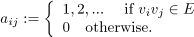 .
.
[2] The incidency matrix of is defined by .
[3] The matrix of weights B = (b_{ij})_{n \times n} of G is defined by b_{ij}:=\left{\begin{array}{l} weight_{k} \quad \mbox{ if } v_{i} v_{j} \in E \\ Inf \quad \mbox{otherwise.} \end{array} \right, where weight_{k} matches weight of k-th edge