TORSCHE Scheduling
Toolbox for Matlab

TORSCHE – Graph Algorithms

Table of Contents

1. List of Algorithms
2. Minimum Spanning Tree
3. Dijkstra's Algorithm
4. Floyd's Algorithm
5. Strongly Connected Components
6. Minimum Cost Flows
7. The Critical Circuit Ratio
8. Hamilton Circuits
9. Graph coloring
10. The Quadratic Assignment Problem

Scheduling algorithms have very close relation to graph algorithms. Scheduling toolbox offer an object graph (see section Chapter 6, Graphs) with several graph algorithms.

1. List of Algorithms

List of algorithms related to operations with object graph are summarized in Table 9.1, “List of algorithms”.

algorithm	command	note
Minimum spanning tree	`spanningtree`	Polynomial
Dijkstra's algorithm	`dijkstra`	Polynomial
Floyd	`floyd`	Polynomial
Minimum Cost Flow	`mincostflow`	Using LP
Critical Circuit Ratio	`criticalcircuitratio`	Using LP
Hamilton circuit	`hamiltoncircuit`	NP-hard
Quadratic Assignment Problem	`qap`	NP-hard

Table 9.1. List of algorithms

2. Minimum Spanning Tree

Spanning tree of the graph is a subgraph which is a tree and connects all the vertices together. A minimum spanning tree is then a spanning tree with minimal sum of the edges cost. A greedy algorithm with polynomial complexity is used to solve this problem (for more details see Demel02). The toolbox function has following syntax:

gmin = spanningtree(g)

gmin: minimum spanning tree represented by graph
g: input graph

>> A = [inf   1  2  inf  7;...
        inf inf  3   4  inf;...
        inf  9  inf  1   1;...
         8   5  inf inf inf;...
         7  inf  4   5  inf];
>> g = graph(A);
>> gmin = spanningtree(g);
>> graphedit(gmin);

Figure 9.1. Spanning tree example

Figure 9.2. Example of minimum spanning tree

3. Dijkstra's Algorithm

Dijkstra's algorithm is an algorithm that solves the single-source cost of shortest path for a directed graph with nonnegative edge weights. Inptut of this algorithm is a directed graph with costs of invidual edges and reference node r from which we want to find shortest path to other nodes. Output is an array with distances to other nodes.

distances = dijkstra(g,r)

g: graph object
r: reference node

>> A = [inf   1  2  inf  7;...
        inf inf  3   4  inf;...
        inf  9  inf  1   1;...
         8   5  inf inf inf;...
         7  inf  4   5  inf];
>> g = graph(A);
>> distances = dijkstra(g,2)

distances =

    11     0     3     4     4

Figure 9.3. Dijkstra's algorithm example

4. Floyd's Algorithm

Floyd is a well known algorithm from the graph theory [Diestel00]. This algorithm finds a matrix of shortest paths for a given graph. Input to the algorithm is an object graph, where the weights of edges are set in UserParam variables of edges. Output is a matrix of shortest paths (U) and optionally matrix of the vertex predecessors (P) in the shortest path and adjacency matrix of lengths (M). Algorithm can be run as follows:

[U,P,M] = floyd(g)

The variable g is an instance of graph object.

5. Strongly Connected Components

The Strongly Connected Components (SCC) of a directed graph are maximal subgraphs for which hold every couple of nodes u and v there is a path from u to v and a path from v to u. For SCC searching Tarjan algorithm is usullay used.

The algorithm is based on depth-first search where the nodes are placed on a stack in the order in which they are visited. When the search returns from a subtree, it is determined whether each node is the root of a SCC. If a node is the root of a SCC, then it and all of the nodes taken off before it form that SCC. The detailed describtion of the algorithm is in [DSVF06]. SCC in a graph G can be found as follows:

scc = tarjan(g)

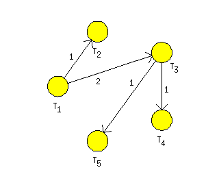
where scc is a vector where the element scc(i) is number of component where the node i belongs to. For graph in Figure 9.5, “A simple network with optimal flow in the fourth user parameter on edges” the algorithm returns fllowing results.

>> tarjan(g)
ans =
     2     2     2     1

Figure 9.4. Strongly Connected Components example.

Figure 9.5. A simple network with optimal flow in the fourth user parameter on edges

6. Minimum Cost Flows

The minimum cost flow model is the most fundamental of all network flow problems. In this problem we wish to determine a least cost shipment of a commodity through a network in order to satisfy demands at certain nodes from available supplies at other nodes [Ahuja93]. Let G=(N,A) be a directed network defined by set N of n nodes and a set A of m directed edges. Each edge (i,j)

TORSCHE Scheduling Toolbox for Matlab