Table of Contents
This chapter presents some case studies fully solvable in the toolbox. Case studies describes the develop process step by step.
This section shows mostly theoretical examples and their solution in the toolbox.
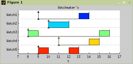
Imagine that you are a man, who repairs watches. Your boss gave you a list of repairs, which have to be done tomorrow. Our goal is to decide, how to organize the work to meet all desired finish times if possible.
List of repairs:
Watch number 1 needs a battery replacement, which has to be finisched at 14:00.
Watch number 2 is missing hand and has to be ready at 12:00.
Watch number 3 has broken clockwork and has to be fixed till 16:00.
The seal ring has to be replaced on watch number 4. It is necessary to reseal it before 15:00.
Watch number 5 has bad battery and broken light. It has to be returned to the customer before 13:00.
Batteries will be delivered to you at 9:00, seal ring at 11:00 and the hand for watch number 2 at 10:00.
Time of repairs:
Battery replacement: 1 hour
Replace missing hand: 2 hours
Fix the clockwork: 2 hours
Seal the case: 1 hour
Repair of light: 1 hour
Let’s look at the list more closely and try to extract and store the information we need to organize the work (see Table 11.1, “Information we need to organize the work”). We consider working day starts at 8:00.
Solution of the case study is shown in five steps:
With formalized information about the work, we can define the tasks.
>> t1=task('Watch1',1,9,inf,14);
>> t2=task('Watch2',2,10,inf,12);
>> t3=task('Watch3',2,8,inf,16);
>> t4=task('Watch4',1,11,inf,15);
>> t5=task('Watch5',2,9,inf,13);
To handle our tasks together, we put them into one object, taskset.
>> T=taskset([t1 t2 t3 t4 t5]);
Our goal is to assign the tasks on one processor, in order, which meets the required duedates of all tasks if possible. The work on each task can be paused at any time, and we can finish it later. In other words, preemption of tasks is allowed. In Graham-Blaziewicz notation the problem can be described like this.
>> prob=problem('1|pmtn,rj|Lmax');The algorithm is used as a function with 2 parameters. The first one is the taskset we have defined above, the second one is the type of problem written in Graham-Blaziewitz notation.
>> TS=horn(T,prob)
Set of 5 tasks
 There is schedule: Horn's algorithm
   Solving time: 0.046875s
Visualize the final schedule by standard
plotfunction, see Figure 11.1, “Result of case study as Gantt chart”.>> plot(TS,'proc',0);
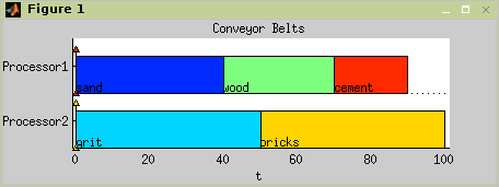
Transportation of goods by two conveyor belts is a simple example of using List Scheduling in practice. Construction material must be carried out from place to place with minimal time effort. Transported articles represent five kinds of construction material and two conveyor belts as processors are available. Table 11.2, “Material transport processing time.” shows the assignment of this problem.
| name | processing time |
|---|---|
| sand | 40 |
| grit | 50 |
| wood | 30 |
| brickc | 50 |
| cement | 20 |
Table 11.2. Material transport processing time.
Solution of the case study is shown in five steps:
Create a
tasksetdirectly through the vector of processing time.>> T = taskset([40 50 30 50 20]);
Since the
tasksethas been created, it is possible to change parameters of all tasks in it.>> T.Name = {'sand','grit','wood','bricks','cement'};Define the problem, which will be solved.
>> p = problem('P|prec|Cmax');Call List Scheduling algorithm with
tasksetand theproblemcreated recently and define the number of processors (conveyor belts).>> TS = listsch(T,p,2) Set of 5 tasks There is schedule: List Scheduling
Visualize the final schedule by standard
plotfunction, see Figure 11.2, “Result of case study as Gantt chart”.>> plot(TS)
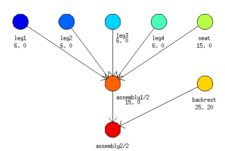
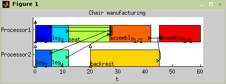
This example is slightly more difficult and demonstrates some of advanced possibilities of the toolbox. It solves a problem of chair manufacturing by two workers (cabinetmakers). Their goal is to make four legs, seat and backrest of the chair and assembly all of these parts with minimal time effort. Material, which is needed to create backrest, will be available after 20 time units of start and assemblage is divided out into two stages. Figure 11.3, “Graph representation of Chair manufacturing” shows the mentioned problem by graph representation.
Solution of the case study is shown in six steps:
Create desired tasks.
>> t1 = task('leg1',6)
 Task "leg1"
  Processing time: 6
  Release time: 0

>> t2 = task('leg2',6);
>> t3 = task('leg3',6);
>> t4 = task('leg4',6);
>> t5 = task('seat',6);
>> t6 = task('backrest',25,20);
>> t7 = task('assembly1/2',15);
>> t8 = task('assembly2/2',15);
Define precedence constraints by precedence matrix
prec. Matrix has sizenxnwherenis a number of tasks.>> prec = [0 0 0 0 0 0 1 0;... 0 0 0 0 0 0 1 0;... 0 0 0 0 0 0 1 0;... 0 0 0 0 0 0 1 0;... 0 0 0 0 0 0 1 0;... 0 0 0 0 0 0 0 1;... 0 0 0 0 0 0 0 1;... 0 0 0 0 0 0 0 0];Create an object of taskset from recently defined objects.
>> T = taskset([t1 t2 t3 t4 t5 t6 t7 t8],prec)
 Set of 8 tasks
  There are precedence constraints
Define solved problem.
>> p = problem('P|prec|Cmax');Call List Scheduling algorithm with taskset and problem created recently and define number of processors and desired heuristic.
>> S = listsch(T,p,2,'SPT')
 Set of 8 tasks
  There are precedence constraints
  There is schedule: List Scheduling
    Solving time: 1.1316s
Visualize the final schedule by standard
plotfunction, see Figure 11.4, “Result of case study as Gantt chart”.>> plot(S)
An real word example demonstrating applicability of the toolbox is shown in the following section.
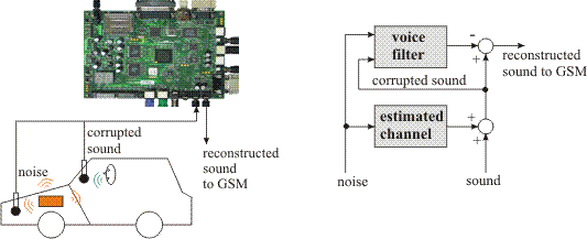
As an illustration, an example application of RLS (Recursive Least Squares) filter for active noise cancellation is shown in Figure 11.5, “An application of Recursive Least Squares filter for active noise cancellation.” [RLS03]. The filter uses HSLA [HSLA02], a library of logarithmic arithmetic floating point modules. The logarithmic arithmetic is an alternative approach to floating-point arithmetic. A real number is represented as the fixed point value of logarithm to base 2 of its absolute value. An additional bit indicates the sign. Multiplication, division and square root are implemented as fixed-point addition, subtraction and right shift. Therefore, they are executed very fast on a few gates. On the contrary addition and subtraction require more complicated evaluation using look-up table with second order interpolation. Addition and subtraction require more hardware elements on the target chip, hence only one pipelined addition/subtraction unit is usually available for a given application. On the other hand the number of multiplication, division and square roots units can be nearly by arbitrary.
RLS filter algorithm is a set of equations (see the inner loop in
Figure Figure 11.6, “The RLS filter algorithm.”) solved in an
inner and an outer loop. The outer loop is repeated for each input data
sample each 1/44100 seconds. The inner loop iteratively processes the
sample up to the N-th iteration (N
is the filter order). The quality of filtering increases with increasing
number of filter iterations. N iterations of the inner
loop need to be finished before the end of the sampling period when output
data sample is generated and new input data sample starts to be
processed.
The time optimal synthesis of RLS filter design on a HW architecture
with HSLA can be formulated as cyclic scheduling on one dedicated
processor (add unit) [Sucha04]. The tasks are constrained by
precedence relations corresponding to the algorithm data dependencies. The
optimization criterion is related to the minimization of the cyclic
scheduling period w (like in an RLS filter application
the execution of the maximum number of the inner loop periods
w within a given sampling period increases the filter
quality).
for (k=1;k<HL;k=k+1)
   E(k)  = E(k-1) - Gfold(k) * Pold(k-1)
   f(k)  = Gold(k-1) * E(k-1)
   P(k)  = Pold(k-1) - Gbold(k) * E(k-1)
   b(k)  = G(k-1) * P(k-1)
   A(k)  = A(k-1) - Kold(k) * P(k-1)
   Gf(k) = Gfold(k) + bnold(k) * E(k)
   F(k)  = L * Fold(k) + f(k) * E(k-1) + T
   B(k)  = L * Bold(k) + b(k) * P(k-1) + T
   fn(k) = f(k) / F(k)
   bn(k) = b(k) / B(k)
   Gb(k) = Gbold(k) + fn(k) * P(k)
   K(k)  = Kold(k) + bn(k) * A(k)
   G(k)  = G(k-1) - bn(k) * b(k)
end
Figure 11.6. The RLS filter algorithm.
Figure 11.6, “The RLS filter algorithm.” shows the inner
loop of RLS algorithm. Data dependencies of this problem can be modeled by
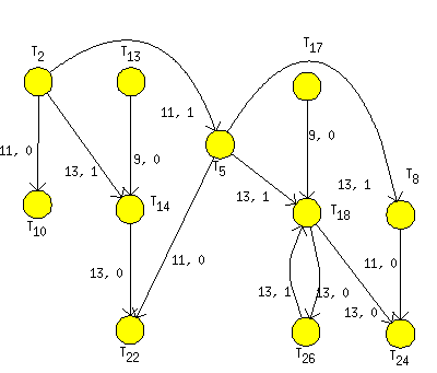
graph rls_hsla in Figure 11.7, “Graph G modeling the scheduling problem on one add unit of
HSLA.”, where nodes represent particular
operations of the RLS filter algorithm on add unit, i.e. a task on the
dedicated processor. First user parameter on node represents processing
time of task (time to `feed' the add unit ). The second one is a number of
dedicated processor (unit). User parameters on edges are lengths and
heights, explained in Section Cyclic scheduling (General).
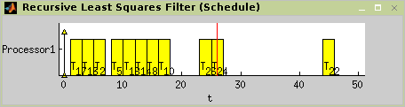
In this case we consider two stages of the filter, i.e. one half of iterations is processed in one stage and second one on the second stage. After processing of the first half of iterations, partial results are passed to the second stage. When the second stage starts to process the input partial results, the first stage starts to process a new sample. Both stages have to share one dedicated processor (add unit), therefore we consider each operation on add unit to be represented by a task with processing time equal to 2 clock cycles. In the first clock cycle an operation of the first stage uses the add unit and in the second clock cycle the add unit is used by the second stage. For more detail see [Sucha04][RLS03] .
Solution of this scheduling problem is shown in following steps:
Load graph of the RLS filter into the workspace (graph
rls_hsla).>> load scheduling\stdemos\benchmarks\dsp\rls_hsla
Transform graph of the RLS filter to graph g weighted by lengths and heights.
>> T = taskset(rls_hsla,'n2t',@node2task,'ProcTime', ...
              'Processor','e2p',@edges2param)
Set of 11 tasks
 There are precedence constraints
Define the problem, which will be solved.
>> prob=problem('CSCH')
 CSCH
Define optimization parameters.
>> schoptions=schoptionsset('verbose',0,'ilpSolver','glpk');Call List Scheduling algorithm with taskset and problem created recently and define number of processors (conveyor belts).
>> TS = cycsch(T, prob, [1], schoptions)
 There are precedence constraints
 There is schedule: General cyclic scheduling algorithm
   Tasks period: 26
   Solving time: 1.297s
   Number of iterations: 1
Visualize the final schedule by standard
plotfunction, see Figure 11.8, “Resulting schedule of RLS filter.”.>> plot(TS,'prec',0);