Table of Contents
TORSCHE is extended with several algorithms and some interfaces to external tools to facilitate develop of scheduling algorithms.
List of the supplementary algorithms is summarized in the following table.
Lot of scheduling algorithms require extra parameters, e.g. parameters of external solvers. To create Scheduling Toolbox structure containing option parameters use
schoptions=schoptionsset('keyword1',value1,'keyword2',value2,...)The function specifies values (V1, V2, ...) of the specific parameters (C1, C2, ...). To change particular parameters use
schoptions=schoptionsset(schoptions,'keyword1',value1,...)
Parameters of Scheduling Toolbox options are summarized in Table 10.2, “List of the toolbox options parameters”. Defauld values of single parameters are typed in italics.
| parameter | meaning | value |
|---|---|---|
| General | ||
maxIter | Maximum number of iterations allowed. | positive integer |
verbose | Verbosity level. | 0 = be silent, 1 = display only critical messages, 2 = display everything |
strategy | Strategy of scheduling algorithm. | This parameter is specific for each scheduling algorithm.
(e.g. listsch algorithm distinguishes 'EST',
'ECT', 'LPT', 'SPT' or a handler of user defined function) |
logfile | Enables logfile creation. | 0 = disable, 1 = enable |
logfileName | Specifies logfile name. | character array |
| Integer Linear Programming (ILP) | ||
ilpSolver | Specifies internal ILP solver (GLPK [Makhorin04], LP_SOLVE [Berkelaar05], CPLEX [CPLEX04], external). | 'glpk', 'lp_solve', 'cplex', 'external' |
extIlinprog | Specifies external ILP solver interface. Specified function
must have the same parameters as function
linprog. | function handle |
miqpSolver | Specifies internal MIQP solver (MIQP [Bemporad04], CPLEX [CPLEX04], external). | 'miqp', 'cplex', 'external' |
extIquadprog | Specifies external MIQP solver interface. Specified
function must have the same parameters as function
linprog. | function handle |
solverVerbosity | Verbosity level of ILP solver. | 0 = be silent, 1 = display only critical messages, 2 = display everything |
solverTiLim | Sets the maximum time, in seconds, for a call to an optimizer. When solverTiLim<=0, the time limit is ignored. Default value is 0. | double |
| Cyclic Scheduling | ||
cycSchMethod | Specifies method for Cyclic Scheduling algorithm. | 'integer', 'binary' |
varElim | Enables elimination of redundant binary decision variables in ILP model. | 0 = disable, 1 = enable |
varElimILPSolver | Specifies another ILP solver for elimination of redundant binary decision variables. | 'glpk', 'lp_solve', 'cplex', 'external' |
secondaryObjective | Enables minimization of iteration overlap as secondary objective. | 0 = disable, 1 = enable |
| Scheduling with Positive and Negative Time-lags | ||
spntlMethod | Specifies an method for spntl
algorithm. | 'BaB' - Branch and Bound, 'ILP' - Integer Linear Programming |
Table 10.2. List of the toolbox options parameters
This supplementary function allows to generate random Data Flow Graph (DFG). It is appointed for benchmarking of scheduling algorithms.
g=randdfg(n,m,degmax,ne)
The function generates Data Flow Graph g, where
relation of node (task) to a dedicated processor is stored in
g.N(i).UserParam. The first parameter
n is the number of nodes in the DFG,
m is the number of dedicated processors. Parameter
degmax restricts upper bound of outdegree of vertices.
Parameter ne is the number of edges.
g=randdfg(n,m,degmax,ne,neh,hmax)
The function with this parameters generates cyclic DFG (CDFG), where
neh is number of edges with user parameter 0 <
g.E(i).UserParam <= hmax. Other
edges has user parameter g.E(i).UserParam=0.
Universal interface for Integer Linear Programming (ILP) allows to call different ILP solvers from Matlab.
[xmin,fmin,status,extra] = ...
   ilinprog(schoptions,sense,c,A,b,ctype,lb,ub,vartype)
Function ilinprog has the following parameters.
Parameter schoptions is Scheduling Toolbox Options
structure (see Scheduling Toolbox Options). The
next parameter sense indicates whether the problem is a
minimization=1 or a maximization=-1. ILP model is specified with column
vector c containing the objective function
coefficients, matrix A representing linear constraints
and column vector b of right sides for the inequality
constraints. Column vector ctype determines the sense
of the inequalities as is shown in Table 10.3, “Type of constraints - ctype.”.
Further, column vector lb
(ub) contains lower (upper) bounds of variables in
specified ILP model. The last parameter is column vector
vartype containing the types of the variables
(vartype(i) = 'C' indicates continuous variable and
vartype(i) = 'I' indicates integer variable).
A nonempty output is returned if a solution is found. Afterwards
xmin contains optimal values of variables. Scalar
fmin is optimal value of the objective function. Value
status indicates the status of the optimization
(1-solution is optimal) and structure extra consisting
of fields time and lambda. Field
time contains time (in seconds) used for solving and
field lambda contains solution of the dual
problem.
Universal interface for Mixed Integer Quadratic Programming (MIQP) allows to call different MIQP solvers from Matlab. This function is very similar to function 'ilinprog', described in section Section 4, “Universal interface for ILP”.
[xmin,fmin,status,extra] = ...
   iquadprog(schoptions,sense,H,c,A,b,ctype,lb,ub,vartype)
Function iquadprog has the following
parameters. Parameter schoptions is Scheduling Toolbox
Options structure (see Scheduling Toolbox Options). The next parameter
sense indicates whether the problem is a minimization=1
or maximization=-1. ILP model is specified with column vector
c and square matrix H containing the
objective function coefficients, matrix A representing
linear constraints and column vector b of right sides
for the inequality constraints. Column vector ctype
determines the sense of the inequalities as is shown in Table 10.4, “Type of constraints - ctype.”.
Further, column vector lb
(ub) contains lower (upper) bounds of variables in
specified MIQP model. The last parameter is column vector
vartype containing the types of the variables
(vartype(i) = 'C' indicates continuous variable and
vartype(i) = 'I' indicates integer variable).
A nonempty output is returned if a solution is found. Afterwards
xmin contains optimal values of variables. Scalar
fmin is optimal value of the objective function. Value
status indicates the status of the optimization
(1-solution is optimal) and structure extra consisting
of fields time and lambda contains
time (in seconds) used for solving and optimal values of dual variables
respectively.
In some versions of Matlab, solver miqp
[Bemporad04] (see Section
Scheduling Toolbox Options) should not find
optimal solution in spite of it exists or can find a solution with worst
value of objective function. When you have a problem with the solver,
please read the miqp solver documentation.
The algorithm requires Optimization Toolbox for Matlab (http://www.mathworks.com/).
CSSIM (Cyclic Scheduling Simulator) is a tool allowing to simulate
iterative loops in Matlab Simulink using TrueTime tool [Cervin06]. The loop described in a language
compatible with Matlab can be transformed into the toolbox structures. In
the toolbox the input iterative loop is scheduled using cyclic scheduling
(see Cyclic scheduling (General)) and optimized iterative
algorithm is transformed into TrueTime code for real-time simulation. The
CSSIM operates in three steps: input file parsing
(function cssimin), cyclic scheduling (see Cyclic scheduling (General)) and True-Time code generation (function
cssimout).
[T,m]=cssimin('dsvf.m');                      %input file parsing

TS=cycsch(T, problem('CSCH'), m, schoptions); %cyclic scheduling

cssimout(TS,'simple_init.m','code.m');        %TrueTime code generation
Input parametr of function cssimin is a string
specifying input file to be parsed. The function returns a taskset
representing the input algorithm. Extra information about algorithm
structure are available in CodeGenerationData structure
contained in TSUserParam of the taskset
T. Further, the function returns the number of
processors, contained in vector m. Function
cssimout generates two files, which are used for
simulation in TrueTime. The first input parameter specifies a taskset
generated using function cssimin, extended with
cyclic schedule. The second parameter specifies name of output TrueTime
initialization file. The third one specifies name of output TrueTime code
of simulated loop.
The language structure of input files is described in the following subsection.
The input file for CSSIM is compatible with Matlab language but it has a simpler and fixed structure. The file is divided into four parts with fixed order: Processors Declaration, Variables Initialization, Iterative Algorithm and Subfunctions.
Processors Declaration: Processors are declared as a structure with fields describing processor parameters. First one is
operatorassigning an operator in the iterative loop to specific processor. Second one isnumberrepresenting number of processors. Following two fields (proctimeandlatency) represent timing parameters of the unit (see section Cyclic scheduling (General)).Example:
struct('operator','+','number',1,'proctime',2,'latency',2);
struct('operator','ifmin','number',1,'proctime',1,'latency',1);
In addition, the simulation frequency for TrueTime can be defined as a structure:
Example:
struct('frequency',10000);
Variables Initialization: The aim of this part is to initialize variables and define input and output variable.
Example:
K = 10;
s2{1} = zeros;
y = num2cell([1 1 1 1 1 1 1 1 1 1]);

struct('output',{'u'},'input','e');
Iterative Algorithm: The input iterative algorithm is described as a loop (for ... end) containing elementary operations (tasks). Each operation is constituted by one line of the loop and can contain only one operation (addition, multiplication, ...).
Example:
for k=2:K-1 ke(k) = e(k) * Kp; s2(k) = c1 + ke(k); s3(k) = ifmax(s2(k),umax); u(k) = ifmin(s3(k),umin); endSubfunctions: The last part contains subfunction called from the iterative algorithm. It usually corresponds to units declared in Arithmetic Units Declaration part. In current version of CSSIM it is used only for simulation of elementary operations. In further version the subfunctions will be also object of the optimization.
Example:
function y=ifmin(a1,a2)
    if(a1<a2)
        y=a2;
    else
        y=a1;
    end
return
Work on this function is still in progress. The authors will be appreciative of any comment and bug report.
For time-exact simulation of schedules of iterative loops TrueTime is used. The scheduled algorithm is simulated using TrueTime Kernels. The CSSIM generates two M-files. First one is an initialization code (simple_init.m) which creates a task for the simulation and initialize variables used in the scheduled algorithm. The second one is a code function (code.m) where each code segment corresponds to a task from the schedule. Lets consider an example of digital state variable filter DSVF06, shown as CSSIM code below
function L=dsvf(I)
%Arithmetic Units Declaration
struct('operator','+','number',1,'proctime',1,'latency',1);
struct('operator','*','number',1,'proctime',3,'latency',3);
struct('frequency',220000);
%Variables Declaration
f = 50;
fs = 40000;
Q = 2;
K = 1000;
F1 = 0.0079; %2*pi*f/fs ||| ??? 2*sin(pi*f/fs)
Q1 = 0.5; %1/Q;
%I = num2cell(simout);
I = ones(1,K);
L = zeros(1,K);
B = zeros(1,K);
H = zeros(1,K);
N = zeros(1,K);
FB = zeros(1,K);
QB = zeros(1,K);
IL = zeros(1,K);
FH = zeros(1,K);
%Iterative Algorithm
for k=2:K
FB(k) = F1 * B(k-1);
L(k) = L(k-1) + FB(k); %L = L + F1 * B
QB(k) = Q1 * B(k-1);
IL(k) = I(k) - L(k);
H(k) = IL(k) - QB(k); %H = I - L -Q1*B
FH(k) = F1 * H(k);
B(k) = FH(k) + B(k-1); %B = F1 * H +B
N(k) = H(k) + L(k); %N = H + L
end
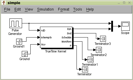
LAfter processing in CSSIM, as shown above, generated files
(simple_init.m and code.m shown bellow) are used in simulation scheme
shown in Figure 10.1, “Simulation scheme with TrueTime Kernel block”. Parameter
Name of init function is set to
simple_init (initialization code).
function simple_init
%
% This file was automatically generated by CSSIM
%

ttInitKernel(1,1,'prioFP');% nbrOfInputs, nbrOfOutputs, fixed priority

data.frequency=220000;    %simulation frequency
data.reg1=0;    % initialization of variable B
data.reg2=0;    % initialization of variable H
data.reg3=0;    % initialization of variable N
data.reg4=0;    % initialization of variable FB
data.reg5=0;    % initialization of variable QB
data.reg6=0;    % initialization of variable IL
data.reg7=0;    % initialization of variable FH
data.reg8=0;    % initialization of variable L
data.const1=50;    % initialization of constant f
data.const2=40000;    % initialization of constant fs
data.const3=2;    % initialization of constant Q
data.const4=1000;    % initialization of constant K
data.const5=0.007900000000000001;    % initialization of constant F1
data.const6=0.5;    % initialization of constant Q1
w=11;
period = w/data.frequency;
deadline = period;
offset = 0;
prio = 1;
ttCreatePeriodictask('task1', offset, period, prio, 'code', data);
function [exectime,data] = code(seg,data) % % This file was automatically generated by CSSIM % i=floor(ttCurrentTime/ttGetPeriod); switch(seg) case 1 data.reg4 = data.const5*data.reg1; % T1 exectime = 3/data.frequency; case 2 data.reg8 = data.reg8+data.reg4; ttAnalogOut(1,data.reg8); % T2 exectime = 0/data.frequency; case 3 data.reg5 = data.const6*data.reg1; % T3 exectime = 1/data.frequency; case 4 data.reg6 = ttAnalogIn(1)-data.reg8; % T4 exectime = 2/data.frequency; case 5 data.reg2 = data.reg6-data.reg5; % T5 exectime = 1/data.frequency; case 6 data.reg7 = data.const5*data.reg2; % T6 exectime = 0/data.frequency; case 7 data.reg3 = data.reg2+data.reg8; % T8 exectime = 3/data.frequency; case 8 data.reg1 = data.reg7+data.reg1; % T7 exectime = 1/data.frequency; case 9 exectime = -1; end
Result of the simulation is shown in Figure 10.2, “Result of simulation”.
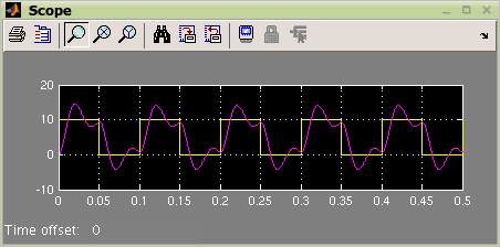
For more details see CSSIM TrueTime demo in the toolbox. For the simulation the TrueTime tool must be installed.
All main objects in TORSCHE can be exported to the XML file format. XML format includes all important information about one or more objects.
XMLSAVE command is used for export to XML for more details see to xmlsave.m.